Edit

Tree-Based Models

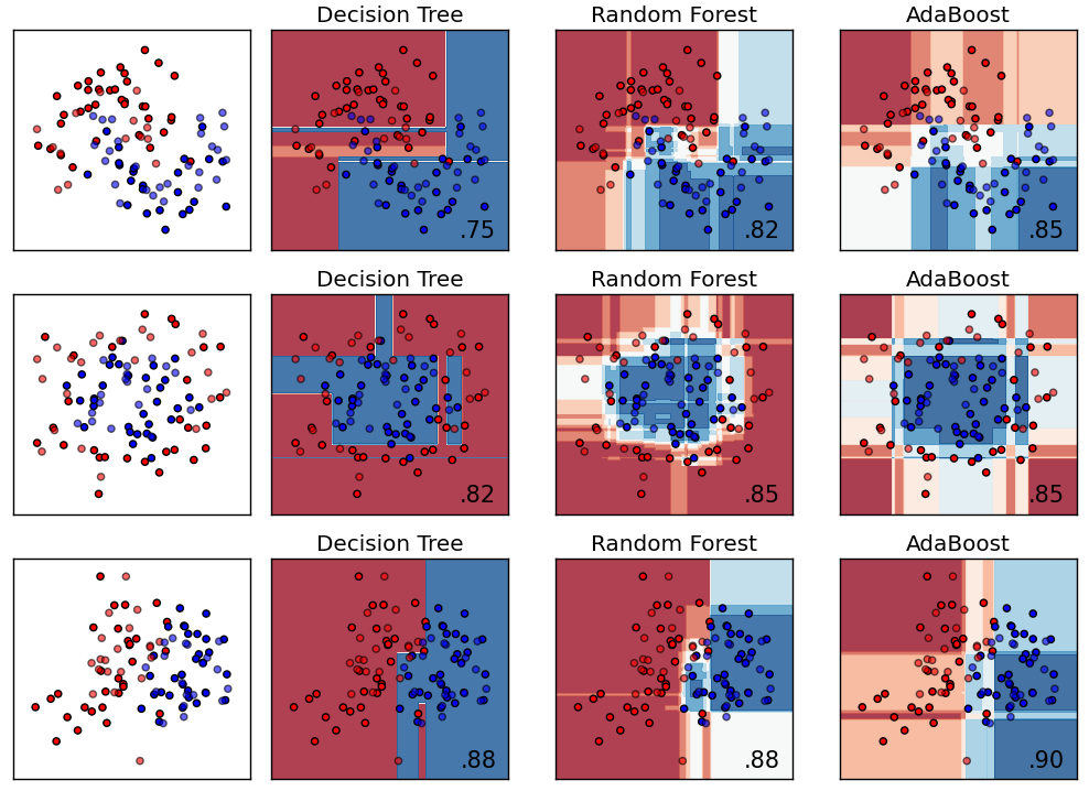
• Tree-based models are models used for classifying non-linearly separable data (like neural networks).
• Applies a “Divide and Conquer” approach by splitting the data into sub-spaces or boxes based on probabilities of outcome.

Credit

Pros

• They are very powerful for tabular data.
• Bring in the capability to handle a dataset with a high degree of errors and missing values.
• Can handle data with both numeric and nominal input attributes.
• Well-known for making no assumptions about spatial distribution.
• Extensively used by banks for loan approvals just because of their extreme transparency.

Cons

• They are weak to capture linear dependencies as it requires a lot of splits.
• Decision trees cannot easily model arbitrary decision boundaries.
• Can only interpolate but not extrapolate.
• Cannot handle large number of features.
• Unfit for incremental learning.
• Have relatively higher error rates — but not as bad as linear regression.
• Often tend to produce wrong results if complex, humanly intangible factors are present.

Decision tree

• At the heart of the popular algorithms for decision tree construction lies the principle of greedy maximization of information gain:
  • At each step the algorithm chooses the variable that gives the greatest information gain i.e., the decrease in entropy upon splitting. $$\large{Gain(S,D)=H(S)-\sum_{V\in{D}}{\frac{|V|}{|S|}H(V)}}$$
  • Entropy is the measure of impurity, disorder or uncertainty in a bunch of examples (the opposite to information). The entropy function is at zero minimum when the probability is \(p=1\) or \(p=0\) with complete certainty. The probability \(p\) is the relative frequency of the outcome. $$\large{H=-\sum{p(x)\log_2{p(x)}}}$$
  • The procedure is repeated recursively until the entropy is zero (or some small value to account for overfitting). Credit
• The simplest heuristics for handling numeric features in a decision tree is to sort its values in ascending order and check only those thresholds where the value of the target variable changes. The value obtained by leaves in the training data is the mean response of observation falling in that region.
• Criterions: In practice, Gini uncertainty and information gain work similarly.
• Introduction to Decision Trees
• A Simple Guide to Entropy-Based Discretization

Pros

• Graphical representation is very intuitive and users can easily relate their hypothesis
• Decision tree is one of the fastest way to identify most significant variables and relation between two or more variables
• Decision trees implicitly perform variable screening or feature selection
• Data type is not a constraint: It can handle both numerical and categorical variables. Can also handle multi-output problems.
• Non-linear relationships between parameters do not affect tree performance
• Fast training and forecasting
• Small number of hyper-parameters

Cons

• Overfitting: Decision-tree learners can create over-complex trees that do not generalize the data well.
• Not fit for continuous variables: While working with continuous numerical variables, decision tree loses information, when it categorizes variables in different categories.
• Small changes to the data can significantly change the decision tree. Decision trees can be unstable because small variations in the data might result in a completely different tree being generated. This is called variance, which needs to be lowered by methods like bagging and boosting.
• Decision tree learners create biased trees if some classes dominate
• The optimal decision tree search problem is NP-complete
• Generally, it gives low prediction accuracy for a dataset as compared to other machine learning algorithms.

Tuning

• A higher value leads to overfitting:
  • max_depth: the maximum depth of the tree.
  • max_features: the maximum number of features with which to search for the best partition (this is necessary with a large number of features because it would be "expensive" to search for partitions for all features).
• A higher value leads to underfitting:
  • min_samples_leaf: the minimum number of samples in a leaf. This parameter prevents creating trees where any leaf would have only a few members.
• Pruning trees. In this approach, the tree is first constructed to the maximum depth. Then, from the bottom up, some nodes of the tree are removed by comparing the quality of the tree with and without that partition (comparison is performed using cross-validation, more on this below).

Random forest

• Random forests are combined through the construction of uncorrelated trees using CART, bagging, and the random subspace method.

Credit

• Bias-variance tradeoff: As random forests training use 1) bootstrap sampling (or sampling with replacement) along with 2) random selection of features for a split, the correlation between the trees (or weak learners) would be low. That means although individual trees would have high variance but the ensemble output will be appropriate (lower variance but the same bias) because the trees are loosely correlated. Thus random forests would give good performance with full depth of decision trees.

Credit

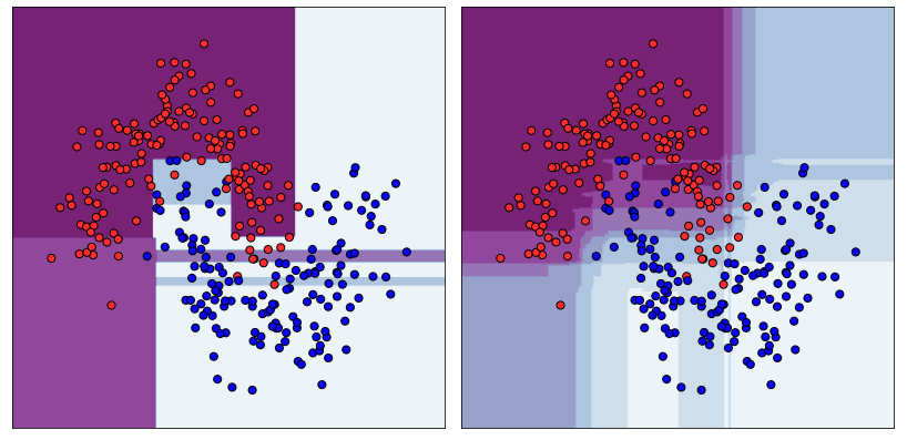
• When bagging with decision trees, we are less concerned about individual trees overfitting the training data. For this reason, the individual decision trees are grown deep and the trees are not pruned.
• To make estimators more independent, ExtraTrees ca be used, which always tests random splits over fraction of features (in contrast to RandomForest, which tests all possible splits over fraction of features).
• After training, predictions for unseen samplescan be made by averaging the predictions from all the individual regression trees or by taking the majority vote in the case of classification trees.
• Parallelized approach:
  • Each tree in forest is independent from the others, so two RF with 500 trees is essentially the same as single RF model with 1000 trees.
• Random forests are mostly used in supervised learning, but there is a way to apply them in the unsupervised setting: Using RandomTreesEmbedding, we can transform our dataset into a high-dimensional, sparse representation. We first build extremely randomized trees and then use the index of the leaf containing the example as a new feature. Under the hood, calculates proximities between pairs of examples that can subsequantly be used in clustering, outlier detection, or interesting data representations.
• Ensembles and Random Forests: A series of notebooks
• Feature Selection Using Random Forests

Pros

• High prediction accuracy; will perform better than linear algorithms in most problems
• Robust to outliers, thanks to random sampling
• Insensitive to the scaling of features as well as any other monotonic transformations due to the random subspace selection
• Doesn't require fine-grained parameter tuning, works quite well out-of-the-box
• Efficient for datasets with a large number of features and classes
• Handles both continuous and discrete variables equally well
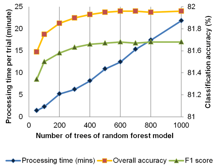
• Rarely overfits. In practice, an increase in the tree number almost always improves the composition. But, after reaching a certain number of trees, the learning curve is very close to the asymptote.

Credit

• There are developed methods to estimate feature importance
• Works well with missing data and maintains good accuracy levels even when a large part of data is missing
• Easily parallelized and highly scalable.

Cons

• The main limitation of Random Forest is that a large number of trees can make the algorithm to slow and ineffective for real-time predictions.
• There are no formal \(p\)-values for feature significance estimation
• Performs worse than linear methods in the case of sparse data: text inputs, bag of words, etc - bagging and suboptimal selection of splits may waste most of the model insight on zero-only areas.
• Unlike linear regression, Random Forest is unable to extrapolate. But, this can be also regarded as an advantage because outliers do not cause extreme values in Random Forests.
• The resulting model is large and requires a lot of RAM
• Overfitting:
  • Prone to overfitting in some problems, especially, when dealing with noisy data.
  • In the case of categorical variables with varying level numbers, random forests favor variables with a greater number of levels. The tree will fit more towards a feature with many levels because this gains greater accuracy.

Tuning

• n_estimators: the number of trees in the forest (the higher the better). A sufficient number of trees can be found by plotting the out-of-bag error (controlled by oob_score) against the number of trees. OOB error is the mean prediction error on each training sample, using only the trees that did not have it in their bootstrap sample.
• A higher value leads to overfitting:
  • max_depth: the maximum depth of the tree. Usually, depth for random forest is higher than for gradient booster.
  • max_features \(m\): the number of features to consider when looking for the best split. For classification problems, it is advisable to set \(m=\sqrt{d}\). For regression problems, we usually take \(m=\frac{d}{3}\), where \(d\) is the number of features.
• A higher value leads to underfitting:
  • min_samples_leaf \(n_{min}\): the minimum number of samples required to be at a leaf node. It is recommended to build each tree until all of its leaves contain only \(n_\text{min}=1\) examples for classification and \(n_\text{min} = 5\) examples for regression.
• Also don't forget to set criterion, random_state and n_jobs.

Boosted trees

• Boosting is an efficient algorithm for converting relatively week learners into a strong learner. A weak learner is defined as one whose performance is at least slightly better than random chance. This technique is called boosting because we expect an ensemble to work much better than a single estimator.
• Sequential approach:
  • In contrast to random forests, boosting is a sequential approach to increase the complexity of models that suffer from high bias, that is, models that underfit the training data.
  • The performance of GBDT model drop dramatically if we remove the first tree as compared to RF.
• Being mainly focused at reducing bias, we will choose most of the time shallow decision trees.
• While this theoretical framework makes it possible to create an ensemble of various estimators, in practice we almost always use GBDT — gradient boosting over decision trees.

Adaptive boosting

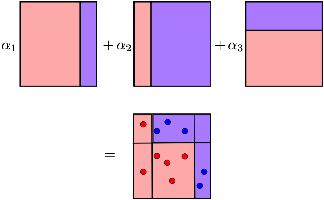
• AdaBoost works by weighting the observations, putting more weight on difficult to classify instances and less on those already handled well. New weak learners are added sequentially that focus their training on the more difficult patterns.
• This process iterate until reached to the specified maximum number of estimators.
• Predictions are made by majority vote of the weak learners’ predictions, weighted by their individual accuracy.

Credit

Pros

• Simple and easy to program
• Few parameters to tune
• No prior knowledge needed about a weak learner
• Provably effective given Weak Learning Assumption

Cons

• AdaBoost works well, but the lack of explanation for why the algorithm is successful sewed the seeds of doubt
• Weak classifiers too complex leads to overfitting when data has strong outliers
• Weak classifiers too weak can lead to low margins, and can also lead to overfitting
• From empirical evidence, AdaBoost is particularly vulnerable to uniform noise

Gradient boosting

• GBDTs train a basic model on the data and then use the previous model’s error as a feature to build successive models.
• Gradient boosting builds an ensemble of trees one-by-one: each decision tree in an ensemble tries to reconstruct the difference between the target function \(f\) and the current predictions of the ensemble \(D\), which is called the residual \(R\), to complement well the existing trees and minimize the training error of the ensemble.

$$\large{R(x)=f(x)-D(x)}$$

• This process sequentially reduces the model’s error because each successive model improves against the previous model’s weaknesses. Each newly trained tree model attempts to linearly separate the remaining, hard to separate, space.
• While in Adaboost shortcomings are identified by high-weight data points, in Gradient Boosting shortcomings (of existing weak learners) are identified by gradients. Here the tree is paying more attention to events with larger module of gradient (those, which were poorly classified on the previous stages).
• Then the predictions \(d\) of the individual trees are summed.

$$\large{D(x)=d_{\text{tree}1}(x)+d_{\text{tree}2}(x)+...}$$

• Before a tree is added to an ensemble, it's predictions are multiplied by learning rate. The larger the learning rate - the larger the contribution made by a single decision tree.
• This process is iteratively carried out until the residuals are zero or until reached to the specified maximum number of estimators.
• GBM produces state-of-the-art results for many commercial (and academic) applications.
• Introduction to Boosted Trees
• Gradient Boosting Interactive Playground

Pros

• Gradient boosting works for generic loss functions, while AdaBoost is derived mainly for classification with exponential loss.
• Can effortlessly return to any point of training process after the ensemble has been already built.

Cons

• AdaBoost can be interepted from a much more intuitive perspective and can be implemented without the reference to gradients by reweighting the training samples based on classifications from previous learners.
• A small change in the feature set or training set can create radical changes in the model
• Not easy to understand predictions

Tuning

• A higher value leads to overfitting:
  • max_depth: the maximum depth of a tree. Increasing it will lead to a faster fitting the dataset but a longer learning time. If the dataset cannot be overfit, there are a lot more of important features and interactions to extract from the data.
  • num_leaves: the number of splits in a tree is very dependent on num_leaves. In fact, higher num_leaves more complex trees GBM can build. The resulting tree can be very deep but have a small number of leaves.
  • subsample, bagging_fraction: controls the fraction of data that will be used at every boosting iteration. The less data is fed, the slower is the training process.
  • colsample_bytree, colsample_bylevel, feature_fraction: Consider only a fraction of features to split on.
  • num_round, num_iterations: The number of rounds (trees) for boosting. With each iteration a new tree is built and added to the ensemble with learning rate as weight. The more steps the model does, the faster it learns.
  • eta, learning_rate: Learning rate, also called shrinkage. One effective way to slow down learning in the gradient boosting model and reduce overfitting is to use a lower learning rate. Both num_round and eta should be tuned simultaneously: We can freeze the learning rate to be reasonably small (0.01) and tune the number of iterations by using early stopping. Then we can do a trick that usually improves the score: multiply num_round by some factor and at the same time divide eta by that factor.
• A higher value leads to underfitting:
  • min_child_weight, min_data_in_leaf: minimum number of instances needed to be in each node (very important). Increasing it will make the model more conservative and regularized. Try a wide range of values depending on data.
  • lambda, lambda_l1: L1 regularization.
  • alpha, lambda_l2: L2 regularization.
• Set random seed to verify that different random states do not change training results much. If results vary a lot, the data may be too random and an extensive cross-validation technique should be used.
• Based on parameters of XGBoost, LightGBM, CatBoost
• Complete Guide to Parameter Tuning in GBMs

Implementations

• Head-to-Head Comparison

XGBoost

• XGBoost is the first GBMT implementation.
• XGBoost achieves overall good results but is significantly slower than its competitors, becoming a bottleneck in iterative design and prototyping widely used on Kaggle.
• It cannot handle categorical features by itself, it only accepts numerical values similar to Random Forest.

LightGBM

• LightGBM improves on XGBoost. The LightGBM paper uses XGBoost as a baseline and outperforms it in training speed and the dataset sizes it can handle. LightGBM is upto 6x faster than XGBoost (used to be 10x faster but XGBoost has caught up) becoming popular on Kaggle where experimentation is important. The accuracies are comparable.
• LGBM does not convert to one-hot coding but uses a special algorithm to find the split value of categorical features.

CatBoost

• Catboost improves over LightGBM by handling categorical features better:
  • By default, CatBoost uses one-hot encoding for features with small number of different values (one_hot_max_size).
  • Frequency encoding as a new feature.
  • Applying mean encoding carelessly results in a target leakage: Catboost introduces an artificial time - a random permutation, and for each instance, it computes its target statistic (mean encoding) based on all previous instances. CatBoost trains several models simultaneously, each of which is trained on a separate permutation.
  • CatBoost also generates combinations of numerical and categorical features.
• CatBoost uses symmetric trees, which are simpler predictors making the algorithm more stable to overfitting.
• No sparse data support yet.
• Overfitting detector: Stops training when the error starts growing on the evaluation dataset.
• Handles missing values out of the box: Creates a separate category for categorical features and uses a constant lower or higher than all other values for numeric features.
• It is also very stable to changing hyperparameters when you have enough training data.
• CatBoost has efficient CPU training implementation. With GPU training it is 2 times faster than LightGBM and 20 times faster than XGBoost. The larger the dataset, the more the speedup.