Optimization
Learning rate
- The learning rate determines how quickly or how slowly you want to update the weights (or parameters).
- Learning rate is one of the most difficult parameters to set:
- It significantly affects model performance. The optimal learning rate is dependent on the topology of the loss landscape, which is in turn depends on both the model architecture and the dataset.
- Try to set a higher learning rate first and then gradually lower it down until the best value is found.
Divergence
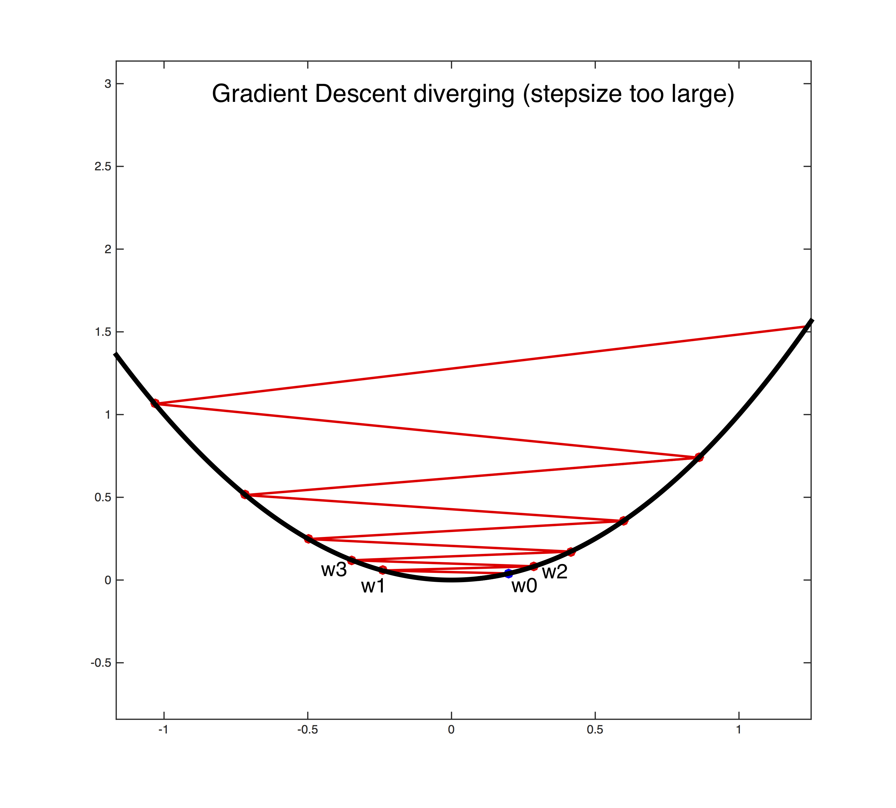
- It's a key differentiator between convergence and divergence.
- If learning rate is set too low, training will progress very slowly as you are making very tiny updates to the weights in the network.
- However, if learning rate is set too high, it can cause undesirable divergent behavior in the loss function.
Local minima
- The best learning rate is associated with the steepest drop in loss.
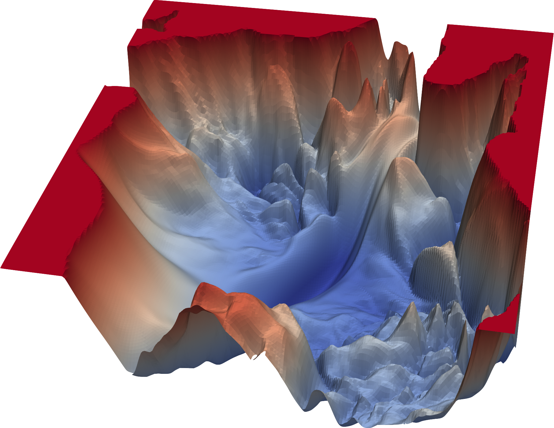
- Recent research has shown that local minima is not neccasarily bad. In the loss landscape of a neural network, there are just way too many minima, and a "good" local minima might perform just as well as a global minima.
- A desirable property of a minima should be it that it should be on the flatter side, because flat minimum are easy to converge to, given there's less chance to overshoot the minima, and be bouncing between the ridges of the minima.
Saddle points
- Another key challenge of minimizing highly non-convex error functions is avoiding getting trapped in their numerous suboptimal local minima.
- Dauphin et al. [3] argue that the difficulty arises in fact not from local minima but from saddle points, i.e. points where one dimension slopes up and another slopes down.
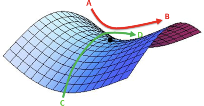
- These saddle points are usually surrounded by a plateau of the same error, which makes it notoriously hard for SGD to escape, as the gradient is close to zero in all dimensions.
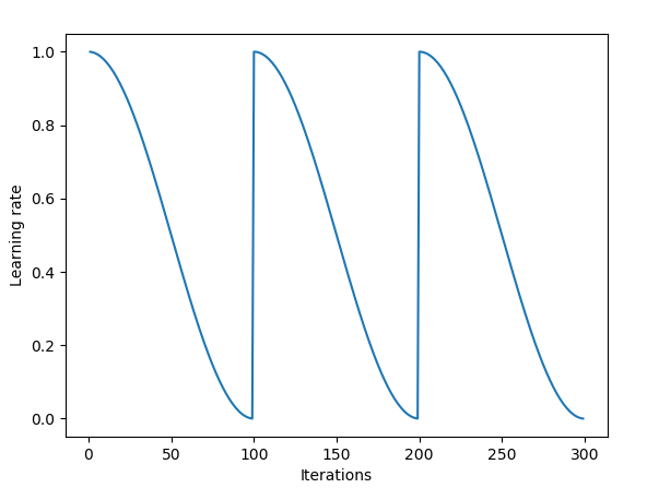
- Tipp: Change the learning rate every iteration according to some (cyclic, validation, etc.) function.
- Cyclical Learning Rates for Training Neural Networks
- A simple decay is not often used for training deep neural networks. Instead, one uses per-parameter decay rates such as RMSProp or Adam or Adamax in order to prevent parameters from languishing on cost plateaus
Gradient descent
- Gradient Descent is used while training a machine learning model to minimize the cost function.
- It is an optimization algorithm, based on a convex function, that tweaks it’s parameters iteratively to minimize a given function to its local minimum.
- Using calculus, we know that the slope of a function is the derivative of the function with respect to a value. This slope always points to the nearest minimum.
$$\large{\theta_{t+1}=\theta_{t}-\alpha\frac{\delta{J(\theta_{t})}}{\delta\theta_{t}}}$$
Pros
- Gradient-based method are very efficient when the search for an optimum happens in an elliptical domain.
Cons
- The objective function might be discontinuous.
- Gradient-based methods are inefficient when the search space solution is large.
- The choice of a starting point conditions the search and the efficiency of a gradient-based method. Converge towards a local minimum is much likely to occur.
Batch gradient descent
- We compute the cost in one large batch computation.
- When computing the cost function we look at the loss associated with each training example and then sum these values together for an overall cost of the entire dataset.
Pros
- Fewer updates to the model means this variant of gradient descent is more computationally efficient than stochastic gradient descent.
- The decreased update frequency results in a more stable error gradient and may result in a more stable convergence on some problems.
- The separation of the calculation of prediction errors and the model update lends the algorithm to parallel processing based implementations.
Cons
- Model updates, and in turn training speed, may become very slow for large datasets.
- Commonly, batch gradient descent is implemented in such a way that it requires the entire training dataset in memory and available to the algorithm.
- Moreover, it begs the question: do we really need to see all of the data before making improvements to our parameter values?
- The updates at the end of the training epoch require the additional complexity of accumulating prediction errors across all training examples.
- The more stable error gradient may result in premature convergence of the model to a less optimal set of parameters.
Mini-batch gradient descent
- It is the most common implementation of gradient descent used in the field of deep learning.
- Mini-batch gradient descent seeks to find a balance between the robustness of stochastic gradient descent and the efficiency of batch gradient descent.
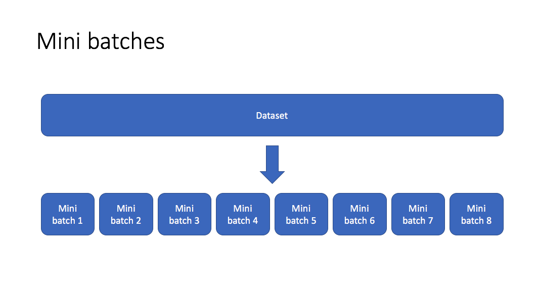
- Allows us to split our training data into mini batches which can be processed individually
- Update your parameters accordingly to the processed mini-batch.
Shuffling
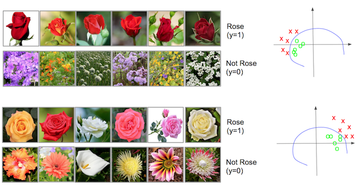
- Every mini-batch used in the training process should have the same distribution
- A difference in the distributions is called the covariate shift
- With every GD iteration, randomize the data before creating mini-batches for images to be uniformly sampled from the entire distribution
Pros
- This allows us to improve our model parameters at each mini batch iteration and take 100 steps towards the global optimum rather than just 1 step
- The model update frequency is higher than batch gradient descent which allows for a more robust convergence, avoiding local minima.
- Makes use of highly optimized matrix optimizations compared to stochastic gradient descent.
- The batching allows both the efficiency of not having all training data in memory and algorithm implementations.
- SGD reaches higher validation accuracy than adaptive learning methods while being slower.
Cons
- Requires three loops:
- Over the number of epochs
- Over the number of iterations
- Over the number of layers
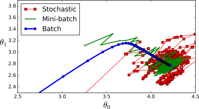
- Vanilla mini-batch gradient descent, however, does not guarantee good convergence.
- Introduces a degree of variance into the optimization process.
- Although we will generally still follow the direction towards the global minimum, we're no longer guarunteed that each step will bring us closer to the optimal parameter values. Advanced optimization techniques are applied here.
- Mini-batch requires the configuration of an additional “mini-batch size” hyperparameter for the learning algorithm.
- Error information must be accumulated across mini-batches of training examples like batch gradient descent.
Best practices
- Common batch sizes (\(m\)) include: 64, 128, 256, and 512.
- Using big batch sizes often leads to overfitting.
- Using small batch sizes achieves the best training stability and generalization performance, for a given computational cost, across a wide range of experiments. In all cases the best results have been obtained with batch sizes \(m=32\) or smaller.
- Very low batch sizes (\(m=2\) or \(m=4\)) may be too noisy and result in underfitting.
- Make sure that a single mini-batch fits into the CPU/GPU memory
- Tune batch size and learning rate after tuning all other hyperparameters.
- It is a good idea to review learning curves of model validation error against training time with different batch sizes when tuning the batch size.
- A rule of thumb: if you increase the batch size by a factor, increase the learning rate by the same factor.
Adaptive learning methods
- Adaptive methods allow to the model to learn and converge faster.
- But in practice, they often lead to overfitting.
Which optimizer to use
- If your input data is sparse, then you likely achieve the best results using one of the adaptive learning-rate methods.
- Also, if you care about fast convergence and train a deep or complex neural network, you should choose one of the adaptive learning rate methods.
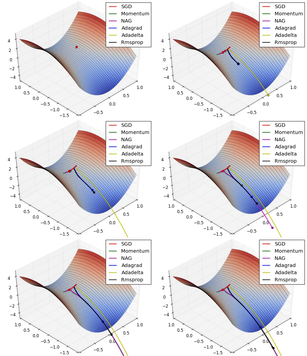
- RMSprop, Adadelta, and Adam are very similar algorithms that do well in similar circumstances.
- Kingma et al. [14:1] show that its bias-correction helps Adam slightly outperform RMSprop towards the end of optimization as gradients become sparser. Insofar, Adam might be the best overall choice. However, it is often also worth trying SGD+Nesterov Momentum as an alternative.
- Many recent papers use vanilla SGD without momentum and a simple learning rate annealing schedule. But it might take significantly longer than with some of the optimizers, is much more reliant on a robust initialization and annealing schedule, and may get stuck in saddle points rather than local minima.
Momentum
- When estimating on a small batch, we’re not always going in the optimal direction, because our derivatives are noisy.
- To prevent gradient descent from getting stuck at local optima (which may not be the global optimum), we can use a momentum term which allows our search to overcome local optima.
- With Momentum update, the parameter vector will build up velocity in any direction that has consistent gradient.
An intuitive understanding of momentum can be painted by a ball rolling down the hill. Its mass is constant all the way, but because of the gravitational pull, its velocity increases over time, making momentum increase. When the directions change, we go marginally slower.
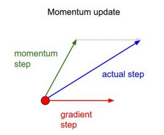
- Momentum takes past gradients into account to smooth out the steps of gradient descent.
$$\large{v_t=\beta v_{t-1}+(1-\beta)g_t}$$
- Exponentially weighed averages can provide us a better estimate which is closer to the actual derivate than our noisy calculations.
| GD with momentum | Beta |
|---|---|
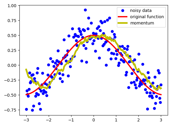 |  |
- The first couple of iterations will provide a pretty bad averages because we don’t have enough values yet to average over.
- The solution is to use the bias-corrected version of velocity.
$$\large{\hat{v}_t=\frac{v_t}{1-\beta^t}}$$
Pros
- SGD with momentum converges slower but the trained network usually generalizes better than Adam.
- It also seems to find more flatter minima.
Best practices
- The velocity is initialized with zeros. So the algorithm will take a few iterations to "build up" velocity and start to take bigger steps.
- If \(\beta=0\), then this just becomes standard gradient descent without momentum.
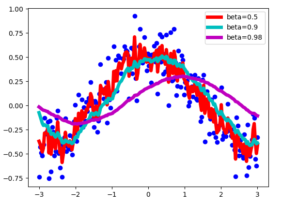
- With bigger values of beta, we get much smother curve, but it’s a little bit shifted to the right
- Common values for \(\beta\) are in \([0.8,0.999]\). If you don't feel inclined to tune this, \(\beta=0.9\) is often a reasonable default.
RMSProp
- RMSProp tries to dampen the oscillations, but in a different way than momentum
- RMSProp implicitly performs simulated annealing. Suppose if we are heading towards the minima, and we want to slow down so as to not to overshoot the minima. RMSProp automatically will decrease the size of the gradient steps towards minima when the steps are too large (Large steps make us prone to overshooting)
- While momentum accelerates our search in direction of minima, RMSProp impedes our search in direction of oscillations.
$$\large{v_t=\beta v_{t-1}+(1-\beta)g_t}$$ $$\large{\theta_{t+1}=\theta_{t}-\alpha\frac{1}{\sqrt{v_t}+\epsilon}g_t}$$
Pros
- The algorithm does well on online and non-stationary problems (e.g. noisy)
- RMSProp is used by DeepMind
Adam
- Adam or Adaptive Moment Optimization algorithm combines the heuristics of both Momentum and RMSProp.
- Adam adds bias-correction and momentum to RMSprop.
Whereas momentum can be seen as a ball running down a slope, Adam behaves like a heavy ball with friction, which thus prefers flat minima in the error surface.
$$\large{v_t=\beta_1v_{t-1}+(1-\beta_1)g_t}$$ $$\large{s_t=\beta_2s_{t-1}+(1-\beta_2)g_t^2}$$ $$\large{\hat{v}_t=\frac{v_t}{1-\beta_1^t}}$$ $$\large{\hat{s}_t=\frac{s_t}{1-\beta_2^t}}$$
$$\large{\theta_{t+1}=\theta_{t}-\alpha\frac{\hat{v}_t}{\sqrt{\hat{s}_t}+\epsilon}g_t}$$
Pros
- In practice, Adam is currently recommended as the default algorithm to use, and often works slightly better than RMSProp.
- It has attractive benefits on non-convex optimization problems
Best practices
- Good default settings for the tested machine learning problems are \(\alpha=0.001\), \(\beta_1=0.9\), \(\beta_2=0.999\) and \(\epsilon=10^{−8}\). The popular deep learning libraries generally use the default parameters recommended by the paper.
LAMB
- Achieves better performance than existing optimizers for a wide range of applications.
- Supports adaptive elementwise updating and layerwise learning rates.
- Enables use of very large batches sizes of 32868; thereby, requiring just 8599 iterations to train.
- LARGE BATCH OPTIMIZATION FOR DEEP LEARNING: TRAINING BERT IN 76 MINUTES
SGDR
- Even though some optimizers try and use ideas of momentum to have the ability to swing out of a local minimum, they are not always that successful.
- We want to encourage our model to find parts of the weight space that are both accurate and stable. Therefore, from time to time we increase the learning rate (this is the "restarts" in SGDR), which will force the model to jump to a different part of the weight space if the current area is "spikey".
