Metric Optimization
- A metric is used to measure the algorithm's performance.
- A loss function is used to optimize an algorithm.
- If a metric is not optimizable:
- Preprocess train and optimize another metric.
- Optimize another metric and postprocess predictions.
- Write a custom loss function.
- Optimize another metric and use early stopping.
- Metrics to Evaluate your Machine Learning Algorithm
- Choosing the Right Metric for Evaluating Machine Learning Models
Tips
- Why is my validation loss lower than my training loss?
- Regularization applied during training, but not during validation/testing.
- Training loss is measured during each epoch while validation loss is measured after each epoch.
- The validation set may be easier than the training set.
Regression metrics
- MSE, RMSE and R-squared are similar from the optimization perspective.
- Do you have outliers (mistakes, measurement errors)? Use MAE
- Do you have unexpected values you should care about? Use (R)MSE
- MSPE and MAPE are sensitive to relative errors and can be thought as weighted versions of MSE and MAE, respectively.
- Relative errors are intended to be both independent of scale and usable on all scales.
- They are mainly used as forecast accuracy measures in time-series data.
- A Survey of Forecast Error Measures
MSE-based metrics
MSE
$$\large{MSE=\frac{1}{n}\sum_{i=1}^{n}{(y_i-\hat{y}_i)^2}}$$
- Mean Squared Error (MSE) measures the average squared difference between the estimated values and what is estimated.
- Can range from 0 to \(\infty\) and are indifferent to the direction of errors.
- It is a negatively-oriented score, which means lower values are better.
- Useful if there are any unexpected values that we should care about.
- MSE is one of the most widely used loss functions because of its ability to partition the variation in a dataset into variation explained by the model and variation explained by randomness.
- Limitations:
- The least useful metric because of the lack of interpretability.
- MSE has the disadvantage of heavily weighting outliers. $$MSE(30, 20)=100$$ $$MSE(30000, 20000)=100000000$$
- Results in a particularly problematic behaviour if applied on noisy data: a single bad prediction may skew the metric towards underestimating the model's quality; if errors are smaller than one, the opposite effect takes place.
- Best constant: mean
- Loss function:
- MSE can be directly optimized and is implemented by most libraries.
- Synonyms: L2 Loss
RMSE
$$\large{RMSE=\sqrt{\frac{1}{n}\sum_{i=1}^{n}{(y_i-\hat{y}_i)^2}}}$$
- Root Mean Square Error (RMSE) is introduced to make scale of the errors to be the same as the scale of targets.
- Expresses average model prediction error in units of the variable of interest.
- Every minimizer of MSE is also a minimizer for RMSE and vice versa, since the square root is an non-decreasing function.
- Even though RMSE and MSE are similar in terms of optimization, they are not interchangeable for gradient-based methods: Travelling along RMSE gradient is equivalent to traveling along MSE gradient but with a different flowing rate.
(R)MSLE
$$\large{L(y,\hat{y})=\frac{1}{n}\sum_{i=0}^{n}{(\log{(y_i+1)}-\log{(\hat{y}_i+1)})^2}}$$
- Mean Squared Logarithmic Error (MSLE) is MSE calculated on logarithmic scale.
- The introduction of the logarithm makes MSLE only care about the relative difference between predictions and target.
$$MSLE(30, 20)=0.02861$$ $$MSLE(30000, 20000)=0.03100$$
- Used in cases where the range of the target value is large (e.g., in forecasting).

- The targets are usually non-negative but can equal to 0 - add a tiny constant before applying log.
- RMSLE is considered as a better metric than MAPE, since it is less biased towards smaller targets.
- Best constant: weighted mean in log space (weights are values themselves)
- Loss function:
- Transform target with \(z_i=\log{y_i+1}\)
- Fit a model with MSE loss
- Transform predictions back with \(\hat{y_i}=\exp{\hat{z_i}}-1\)
R squared
$$\large{R^2=1-\frac{SS_{\text{RES}}}{SS_{\text{TOT}}}=\frac{\sum_i{(y_i-\hat{y}_i)^2}}{\sum_i{(y_i-\overline{y}_i)^2}}}$$
- The coefficient of determination, or \(R^2\) measures how much the model is better than the naive MSE baseline.
- The MSE baseline can be thought of as the MSE that the simplest possible model would get.
- Has the advantage of being scale-free (values between \(-\infty\) and \(1\)).
- Values outside the range can occur when the model fits the data worse than the baseline.
- Limitations:
- R-squared cannot determine whether the coefficient estimates and predictions are biased.
- Low values are not inherently bad for harder-to-predict data while high values do not necessarily indicate that the model has a good fit.
- \(R^2\) will never decrease as variables are added and will probably experience an increase due to randomness. The adjusted R-squared can solve this by increasing only if the new term improves the model more than would be expected by chance.
- Best constant: mean
- Loss function:
- RMSE or MSE loss should be used instead.
MAE-based metrics
MAE
$$\large{MAE=\frac{\sum_{i=1}^{n}{|y_i-\hat{y}_i|}}{n}}$$
- MAE measures the average magnitude of the errors in a set of predictions, without considering their direction.
- Expresses average model prediction error in units of the variable of interest.
- Can range from 0 to \(\infty\) and are indifferent to the direction of errors.
- It is a negatively-oriented score, which means lower values are better.
- The individual differences are weighted equally.
- MAE loss is useful if the training data is corrupted with outliers.
- It is widely used in finance, where error 10 is exactly two times worse than error 5.
- If the absolute value is not taken, the average error becomes the Mean Bias Error (MBE).
- Best constant: median (more robust to outliers than mean)
- Loss function:
- MAE can be directly optimized but is implemented by fewer libraries.
- Not differentable when predictions are equal to target (rare case)
- One big problem in using MAE loss (for neural nets especially) is that its gradient will be large even for small loss values. Here helps a dynamic learning rate which decreases as we move closer to the minima.
- MAE criterion is slower than MSE criterion
- Synonyms: L1 Loss, Median regression
MAE vs. RMSE
- RMSE has a tendency to be increasingly larger than MAE as the test sample size increases.
- RMSE has the benefit of penalizing large errors more.
- MAE is the most robust choice in respect to outliers.
- MAE is shown to be an unbiased estimator while RMSE is a biased estimator.
- Loss functions:
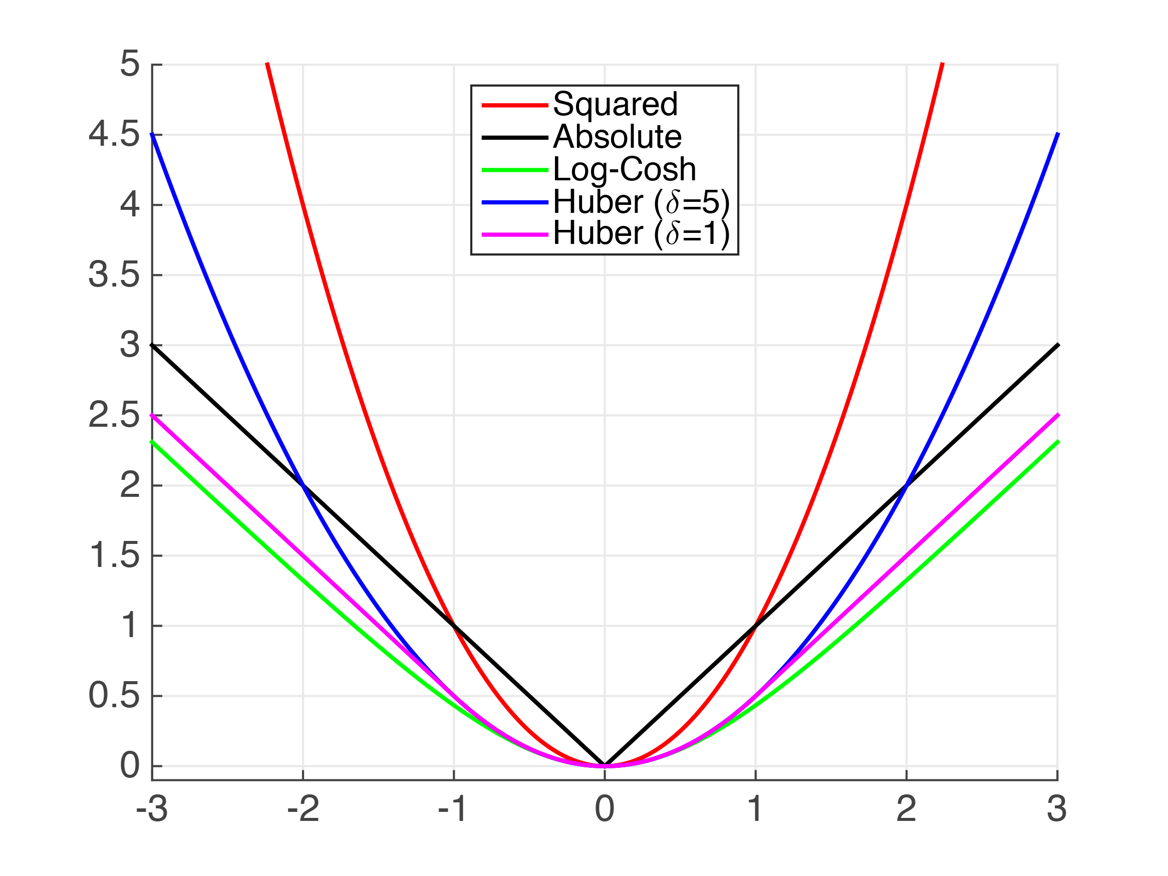
- L1 loss is more robust to outliers, but its derivatives are not continuous, making it inefficient to find the solution.
- L2 loss is sensitive to outliers, but gives a more stable and closed form solution (by setting its derivative to 0.)
- Comparing the performance using L1 loss and L2 loss
- As option: Huber loss combines good properties from both MSE and MAE.
- As another option: Log-Cosh loss has all the advantages of Huber loss, and it’s twice differentiable everywhere (which is more favorable for models using Newton’s method), unlike Huber loss.

Credit
MAPE
$$\large{MAPE=100\frac{1}{n}\sum_{i=1}^{n}{\frac{|y_i-\hat{y}_i|}{y_i}}}$$
- Mean Absolute Percentage Error (MAPE) or Mean Absolute Deviation (MAD) is relative MAE (in %).
- MAPE is often preferred because apparently managers understand percentages better than squared errors.
- It is also commonly used as a loss function for regression problems and in model evaluation because of easy interpretation.
- MAPEs greater than 100% can occur.
- Limitations:
- MAPE is biased towards smaller targets which yield higher errors.
- MAPE can't be used for values where divisions and ratios make no sense (temperature scales).
- RMSE method is more accurate and recent.
- Best constant: weighted median
- Loss function:
- Use weights for samples (
sample_weight) and optimize MAE. - Or resample the dataset beforehand (
df.sample) and optimize MAE. - Usually need to resample many times and average.
- Use weights for samples (
Classification metrics
- Logloss is the only metric that is easy to optimize directly.
- For a binary classification task, fit any metric, and tune with the binarization threshold.
- For multi-class tasks, fit any metric and tune parameters comparing the models by their accuracy score (not optimization metric).
Accuracy
$$\large{Accuracy=\frac{1}{n}\sum_{i=1}^{n}{[y_i=\hat{y}_i]}}$$
- Accuracy is the ratio of number of correct predictions to the total number of input samples.
- Works well for balanced datasets (one can get a nearly perfect score with imbalanced data classes).
- To compute accuracy we need hard predictions, that is, apply a threshold.
- The optimal threshold can be found with grid search.
- Best constant: the most frequent class
- Loss function:
- The loss function is not differentable since gradients are zero almost always.
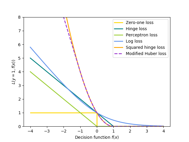
- Zero-one loss may be approximated with a proxy loss such as logloss or Hinge loss.

Credit
Dealing with imbalanced data
- Resampling:
- Undersampling: sample from the majority class
- Oversampling: replicate points from the minority class
- Consider testing random and non-random (e.g., stratified) sampling schemes.
- Consider testing different resampled ratios.
- Generating synthetic data: create new synthetic points from the minority class or both classes (see SMOTE).
- But information about class distribution is lost when resampling the dataset and can skew predictions on test.
- Penalize mistakes on minority classes with class re-weighting (
sample_weight). - Use a different performance metric (e.g., precision, recall, F-score, ROC AUC).
- What metrics should be used for evaluating a model on an imbalanced data set?
- Hands-on example: Detecting credit card fraud
LogLoss
$$\large{LogLoss=-\frac{1}{n}\sum_{i=1}^{n}\sum_{j=1}^{n}{y_{i,j}\log{\hat{y}_{i,j}}}}$$
- Logarithmic loss, or logloss, increases as the predicted probability diverges from the actual label.
- For all samples, enforces the model to assign a probability to be of a certain class.
- To ensure numeric stability, predictions are clipped to be from \([10^{-15}, 1-10^{-15}]\) instead of \([0, 1]\).
- Logloss has no upper bound (\([0, \infty)\)) with smaller values indicating a better fit.
- Best constant: class frequency as vector
- Loss function:
- Logloss can be directly optimized and is implemented by most libraries.
- NNs at default optimize logloss for classification.
- Random forest classifiers are bad at logloss and produce rather conservative predictions. RFs can be calibrated in several ways: 1) Platt scaling (fit logistic regression to predictions), 2) isotonic regression, and 3) stacking.
- Calibrated classifiers (rarely the case) will return posterior probabilities where threshold 0.5 would be optimal.
AUC
- Area under the ROC Curve (AUC) of a classifier is a performance measurement for classification problem at various thresholds settings.
- AUC tells how much model is capable of distinguishing between classes 0 and 1.

- AUC is a rank-based metric (depends on ordering of predictions, not on absolute values)
- Used for binary classification problems.
- For multi-class tasks, we can plot \(N\) number of AUC-ROC curves for \(N\) number classes using one-vs-all methodology.
- Good for cases when you need to estimate how well your model is at discriminating TRUE from FALSE values.
- Removes the need for hard predictions and dependency on the threshold.
- AUC can be obtained in different ways:
- Area under the curve of plot FPR (\(\frac{TP}{TP+FN}\)) vs TPR (\(\frac{FP}{FP+TN}\)) at different points in \([0, 1]\) (Understanding ROC curves)
- The probability of a pair of the predictions to be ordered in the right way.
- The expectation that the classifier will rank a randomly chosen positive higher than a randomly chosen negative.
- Best constant: any constant, random predictions lead to \(AUC=0.5\)
- Loss function:
- Although the loss function of AUC has zero gradients almost everywhere, exactly as accuracy loss, there exists an algorithm to optimize AUC with gradient-based methods, which use pair-wise loss instead of point-wise loss (supported by LGBM, XGBoost).
- XGBoost learned with logloss gives a comparable AUC score.
Cohen's Kappa
$$\large{\kappa=1-\frac{1-p_{\text{observed}}}{1-p_{\text{chance}}}}$$
- The kappa statistic is a metric that compares an observed accuracy with an expected accuracy (random chance). An accuracy of 80% is a lot more impressive with an expected accuracy of 50% versus an expected accuracy of 75%.
- It is used not only to evaluate a single classifier, but also to evaluate classifiers amongst themselves.
- Outputs 0 for baseline accuracy and 1 for excelent accuracy.
- The more complex (and random) the dataset is, the lower kappa will be considered as high enough (such as 0.4)
- Similar to how R squared better scales the MSE values for being easier explained.
- Kappa is quite intuitive for medicine applications: how much the model agrees with professional doctors?
- Best constant: the most frequent class
- Loss function:
- Treat this task as a regression problem (but more complex than MSE) and post-process the predictions by rounding them with a (tuned) threshold (if we relax the predictions to take values between the labels).
- Or implement "soft kappa" loss
Ranking metrics
- Learning to Rank using Gradient Descent -- original paper about pairwise method for AUC optimization
- Overview of further developments of RankNet
- RankLib (implementations for the 2 papers from above)
- Learning to Rank Overview