Convolutional Neural Networks
- Convolutional networks make explicit assumptions on the structure of the input that allow them to encode certain properties in their architecture. These choices make them efficient to implement and vastly reduce the amount of parameters in the network.
- Convolutional Neural Networks (CNNs / ConvNets)
- Visualizing and Understanding Convolutional Networks (2013)
- Visualization with Keras.js
Visual cortex
- Convolutional neural networks are biologically inspired variants of multilayer perceptrons that are designed to emulate the behavior of a visual cortex.
- There are two basic visual cell types in the brain:
- simple cells, whose output is maximized by straight edges having particular orientations within their receptive field.
- complex cells, which have larger receptive fields, whose output is insensitive to the exact position of the edges in the field.
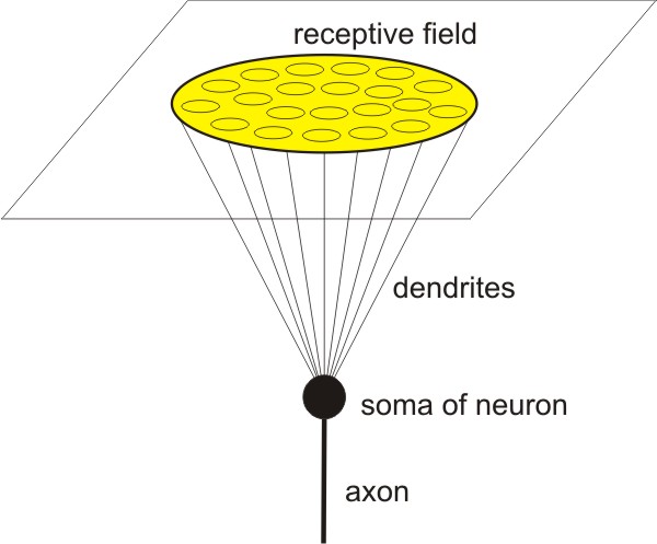
- In vision, a receptive field of a single sensory neuron is the specific region of the retina in which something will activates that neuron.
- Neighboring cells have similar and overlapping receptive fields.
- The neocortex stores information in sequences of patterns, hierarchically.

Feature extraction
- The most fundamental advantage of a convolutional neural network is automatic feature extraction for the given task; provided that the input can be represented as a tensor in which local elements are correlated with one another.
- They also take into consideration the N-dimensional structure of the input.
- CNNs take advantage of local spatial coherence in the input, which allow them to have fewer weights as some parameters are shared. This process, taking the form of convolutions, makes them especially well suited to extract relevant information at a low computational cost.

- In image classification a CNN may
- learn to detect edges from raw pixels in the first layer,
- then use the edges to detect simple shapes in the second layer,
- then use these shapes to detect higher-level features (such as facial shapes in higher layers),
- and then classify these high-level features.
Layers
- CNN is made up of layers. Every layer has a simple API:
- It transforms an input volume to an output volume with some differentiable function that may or may not have parameters.
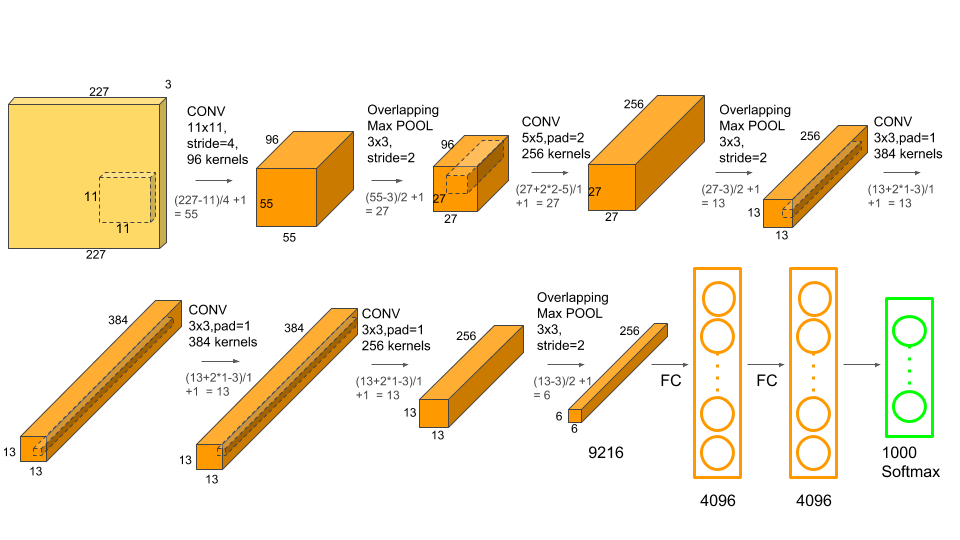
- CNN consists of an input and an output layer, as well as multiple hidden layers. The hidden layers of a CNN typically consist of convolutional layers, pooling layers, fully connected layers and normalization layers.
- You can think of each convolution operation as detecting a specific feature (i.e., if the input contains vertical edges).
- By performing the pooling operation you are keeping information about whether or not the feature appeared in the input, but you are losing global information about locality, thus compressing the input.
- Finally, the fully-connected layer performs classification.
 Credit
Common patterns
- As you go deeper, the height and width of matrices decrease and the number of channels (depth) increases, because each layer extracts a feature from the matrix and stores it in a separate channel
- Usually, the CONV layers preserve the spatial size of their input, while the POOL layers alone are in charge of down-sampling the volumes spatially.
- Activation size tends to go down gradually.
- At the end there are a couple of fully-connected layers.
- Most parameters are stored in fully-connected layers.
- The number of layers is usually the number of layers that have parameters.
Input layer (INPUT)
- INPUT holds the raw pixel values of the image:
- For example, input of 32x32x32 encodes an image of width 32, height 32, and three color channels R,G,B.
 Credit
- For example, input of 32x32x32 encodes an image of width 32, height 32, and three color channels R,G,B.
- Channels are different "views" on input data:
- For example, in image recognition you typically have RGB channels.
- In NLP you could have a channel for the same sentence represented in different languages, or phrased in different ways.
- Generally, the number of channels can be in the hundreds, rather than just RGB or RGBA.
Sizing pattern
- The input layer (that contains the image) should be divisible by 2 many times:
- Common numbers include 32 (e.g. CIFAR-10), 64, 96 (e.g. STL-10), or 224 (e.g. common ImageNet ConvNets), 384, and 512.
Convolutional layer (CONV)
- The primary purpose of convolution is to extract features from the input volume.
- Convolution operation captures the local dependencies in the original data.
- Pixels close to each other are likely to be semantically related (part of the same object).
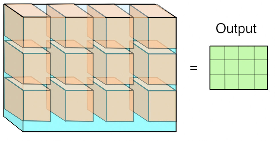
- Convolution is performed on the input volume with the use of a sliding window to then produce an output volume.
- The sliding window is also called a kernel, filter, or feature detector.
- The area of the filter is inspired from the receptive field and called a patch.
- Filter can be used for blurring, sharpening, embossing, edge detection, and more.
- Feature detector is applied on input image to produce a feature map.

- In contrast to traditional networks, we use convolutions (mathematically "cross-correlation") over the dot product.
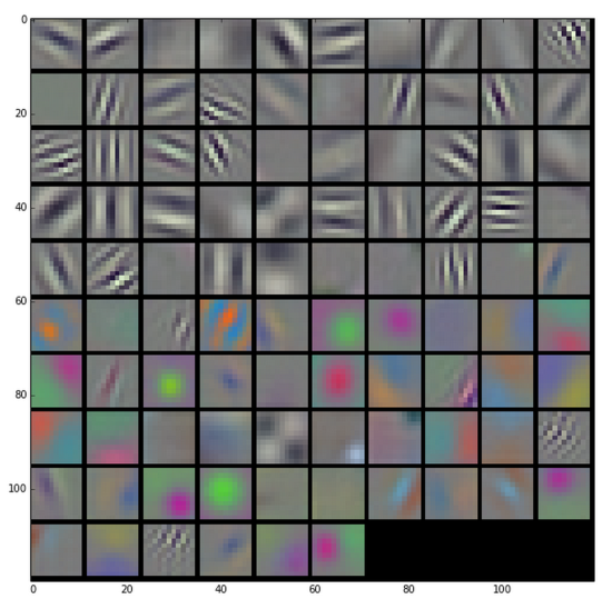
- The convolution operation produces its output by taking a number of "kernels" of weights and applying them across the image.
- Each kernel is another three-dimensional array of numbers, with the depth the same as the input image, but with a much smaller width and height, typically something like 7×7.
- To produce a result, a kernel is applied to a grid of points across the input image.
- At each point where it’s applied, all of the corresponding input values and weights are multiplied together, and then summed to produce a single output value at that point.

- You can think of this operation as something like an edge detector:
- The kernel contains a pattern of weights, and when the part of the input image it’s looking at has a similar pattern it outputs a high value.
- When the input doesn’t match the pattern, the result is a low number in that position.
- Because the input to the first layer is an RGB image, all of these kernels can be visualized as RGB too, and they show the primitive patterns that the network is looking for.

- During the training phase, a CNN automatically learns the values of its kernels.
Pros
- Location Invariance:
- Let’s say you want to classify whether or not there’s an elephant in an image. Because you are sliding your filters over the whole image you don’t really care where the elephant occurs.
- Compositionality:
- Each filter composes a local patch of lower-level features into higher-level representation. It makes intuitive sense that you build edges from pixels, shapes from edges, and more complex objects from shapes.
- Local connectivity:
- When dealing with high-dimensional inputs such as images, it is impractical to connect neurons to all neurons in the previous volume.
- Instead, we will connect each neuron to only a local region of the input volume.
- The connections are local in space (along width and height), but always full along the entire depth of the input volume.
- Parameter sharing:
- All neurons in a single depth slice use the same weight vector
- Note that sometimes the parameter sharing assumption may not make sense. This is especially the case when the input images have some specific centered structure. In that case it is common to relax the parameter sharing scheme, and instead simply call the layer a Locally-Connected Layer.
- Sparsity of connections:
- In each layer, each output value depends only on a small number of inputs
- Convolutions are a central part of computer graphics and implemented on a hardware level on GPUs.
Sizing pattern
- The conv layers should use small filters (e.g. 3x3 or at most 5x5), use a stride of \(S=1\), and crucially, padding the input volume with zeros in such way that the conv layer does not alter the spatial dimensions of the input.
- A larger kernel is preferred for information that is distributed more globally, and a smaller kernel is preferred for information that is distributed more locally.
Hyperparameters
- Unlike a regular network, the layers of a ConvNet have neurons arranged in 3 dimensions: width, height, depth.

- The size of the output map depends on multiple hyperparameters:
$$\large{\text{output width}=\frac{W-F_w+2P}{S_w}+1}$$
$$\large{\text{output height}=\frac{H-F_h+2P}{S_h}+1}$$
where \(W\): input width, \(H\): input height, \(F\): filter size, \(P\): padding, \(S\): stride size
Depth
- The number of filters to use for the convolution operation.
- We refer to a set of neurons that are all looking at the same region of the input as a depth column.
- The more number of filters we have, the more image features get extracted.
Stride
- Stride defines by how much to shift the filter at each step.
- A larger stride size leads to fewer applications of the filter and produce smaller output volumes spatially.
Zero-padding
- Sometimes, it is convenient to pad the input matrix with zeros around the border, so that we can apply the filter to bordering elements of our input image matrix.
- The nice feature of zero padding is that it will allow us to control the spatial size of the output volumes.
- Adding zero-padding is also called wide convolution, and not using zero-padding would be a narrow convolution.
ReLU layer (RELU)
- Convolution is a linear operation due to element-wise matrix multiplication and addition, so we have to account for non-linearity by introducing a non-linear function like ReLU.
- The output volume is also referred to as the rectified volume.
- RELU layer leaves the size of the volume unchanged.
Pooling layer (POOL)
- Spatial Pooling (also called subsampling or downsampling) reduces the dimensionality of each volume but retains the most important information.
- Its function is to progressively reduce the spatial size of the representation to reduce the amount of parameters and computation in the network.
- Pooling layer downsamples the volume spatially, independently in each depth slice of the input volume.

- Spatial pooling can be of different types. Max pooling used much more often than other types.
Pros
- Makes the input representations (feature dimension) smaller and more manageable.
- Reduces the number of parameters and computations in the network, therefore, controlling overfitting.
- Makes the network invariant to small transformations, distortions and translations in the input image.
Cons
- A larger stride in CONV layers can be used to discard pooling layers.
- Discarding pooling layers has also been found to be important in training good generative models, such as variational autoencoders (VAEs) or generative adversarial networks (GANs).
- It seems likely that future architectures will feature very few to no pooling layers.
Sizing pattern
- The most common setting is to use max-pooling with 2x2 receptive fields (i.e. \(F=2\)), and with a stride of 2 (i.e. \(S=2\)).
- Note that this discards exactly 75% of the activations in an input volume.
- It is very uncommon to see receptive field sizes for max pooling that are larger than 3 because the pooling is then too lossy and aggressive - this usually leads to worse performance.
Fully-connected layer (FC)
- The purpose of the fully-connected layer is to perform classification (or regression) tasks.
- Apart from classification, adding a fully-connected layer is also a (usually) cheap way of learning non-linear combinations of these features.
CONV vs FC
- It is worth noting that the only difference between FC and CONV layers is that the neurons in the CONV layer are connected only to a local region in the input, and that many of the neurons in a CONV volume share parameters.
- It turns out that it’s possible to convert between FC and CONV layers:
- For any CONV layer there is an FC layer that implements the same forward function.
- The weight matrix would be a large matrix that is mostly zero except for at certain blocks (due to local connectivity) where the weights in many of the blocks are equal (due to parameter sharing).
Constraints
- The largest bottleneck to be aware of when constructing CNNs is the (GPU) memory bottleneck.
- There are three major sources of memory to keep track of:
- the raw number of activations at every layer,
- the network parameters, their gradients, and commonly also a step cache of an optimization algorithm,
- miscellaneous memory such as the image data batches, perhaps their augmented versions, etc.
- If your network doesn’t fit, a common heuristic to “make it fit” is to decrease the batch size, since most of the memory is usually consumed by the activations.
- In practice, people prefer to make the compromise at only the first CONV layer of the network.