Edit

Linear Models

• In linear models, the relationships are modeled using linear predictor functions.
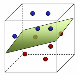
• Linear methods split space into 2 subspaces.

Credit

Pros

• Linear models are frequently favorable due to their interpretability and often good predictive performance.
• Linear regression is often not computationally expensive.
• They are easily comprehensible and transparent in nature.
• Can handle a very large number of features, especially with very low signal to noise ratio.
• Can be used if covariate shift is likely.

Cons

• They strongly rely on a linear relationship.
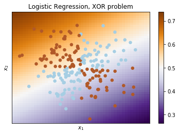
• The most famous toy example of where classes cannot be divided by a hyperplane (or line) with no errors is "the XOR problem". But if one were to give polynomial features as an input, then the problem can be solved.

Credit

• Weaker than other algorithms in terms of reducing error rates.
• Rely on continuous data to build regression capabilities.
• Each missing value removes one data point that could optimize the regression.
• Outliers can significantly disrupt the outcomes.

Regression

• In regression analysis, the coefficients \(w\) in the regression equation are estimates of the actual population parameters.

$$\large{y=\beta_01+\beta_1*x_1+...+\beta_px_p+\epsilon=Xw+\epsilon}$$

• Regression analysis:
  • Indicates the significant relationships between dependent variables and independent variable.
  • Indicates the strength of impact of multiple independent variables on a dependent variable.
  • Compares the effects of variables measured on different scales.

Solution approaches

• Solving the model parameters analytically using closed-form equations (LinearRegression)
• Using an optimization algorithm such as SGD, Newton's method, etc. (SGDRegressor)
  • Optimization algorithms are particularly useful when the number of samples (and features) is very large.

Tuning

• Construct validation curves to compare the results depending on the complexity of the model (validation_curve):
  • if the two curves are close to each other and both errors are large, it is a sign of underfitting.
  • if the two curves are far from each other, it is a sign of overfitting.
• Construct learning curves to compare the results depending on the number of observations (learning_curve):
  • The parameters of the model are fixed in advance.
  • if the curves converge, adding new data won't help, and it is necessary to change the complexity of the model.
  • if the curves have not converged, adding new data can improve the result.

Linear regression

OLS

• The OLS (ordinary least squares) is used to estimate the coefficients in a linear regression model by minimizing the sum of squares of the differences between fitted values and observed values regardless of the form of the distribution of the errors.
• To solve this optimization problem, we need to calculate derivatives with respect to the model parameters.

$$\large\min_w||y-\hat{y}||^2_2$$

• The OLS estimator has the desired property of being unbiased. However, it can have a huge variance when
  • The predictor variables are highly correlated with each other.
  • There are many predictors (independent variables).
• The OLS approach can be used to fit models that are not linear models.
• When the assumptions are met, OLS regression can be more powerful than other regression methods.
• The parametric form makes it relatively easy to interpret.
• Challenges:
  • OLS cannot distinguish between variables with little or no influence.
  • These variables distract from the relevant regressors.
  • Least squares perform badly in the presence of outliers.
  • Redundant features may unnecessarily degrade the performance.

MLE

• Maximum likelihood estimation (MLE) can be used to estimate parameters if the form of the distribution of the errors is known.
• The ML estimator is identical to the OLS estimator given that errors are normally distributed.

Assumptions

• We assume that
  • the relationship between dependent and independent variables is linear and additive,
  • the observations are independent of one another (no autocorrelation),
  • the explanatory variables are independent of each other (no multicollinearity),
  • the errors, or residuals, are independent of time, predictions or independent variables (homoscedasticity),
  • and the distribution of residuals is normal.
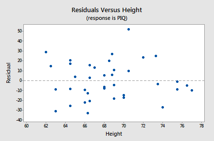
• If a linear model makes sense, the residuals will (using residual-by-predicted plot)
  • have a constant variance,
  • be approximately normally distributed (with a mean of zero), and
  • be independent of one another.
• The best way to assess assumptions is by using residual plots. Credit
• The Gauss-Markov theorem states that OLS produces best estimates when the assumptions hold true. Also, as the sample size increases to infinity, the coefficient estimates converge on the actual population parameters.
• Many of the assumptions describe properties of the error terms.
• We use residuals of a fitted model instead, which are the sample estimate of the error for each observation.
• If the residuals also follow the normal distribution, we can safely use hypothesis testing to determine whether the independent variables and the entire model are statistically significant. We can also produce reliable confidence intervals and prediction intervals.
• Regression Model Assumptions

Regularization

• There are situations where we might reduce variance at the cost of introducing some bias for the sake of stability.
• To decrease the model complexity, one can
  • pick only a subset of all \(p\) variables which is assumed to be relevant,
  • project \(p\) predictors into a \(d\)-dimensional subspace with \(d<p\),
  • or shrink large coefficients towards zero.
• Regularization methods add a penalty to the OLS formula.
• Cross-validation finds the best approach for a given dataset.

Ridge regression

• Ridge regression decreases the complexity by keeping the variables but penalizing them if they are far from zero.
• Ridge penalizes sum of squared coefficients (the so-called L2 penalty).

$$\large\alpha||w||^2_2$$

• Setting \(\alpha\) to 0 is the same as using the OLS.
• Ridge regression can shrink parameters close to zero.
• Solves the multicollinearity issue:
  • The greater the amount of shrinkage \(\alpha\), the more robust the coefficients become to collinearity.
  • The coefficients of correlated predictors are similar.
• Penalization term \(\alpha\) can be chosen by performing cross-validation (RidgeCV).
• Ridge performs well when most predictors impact the response.
• Ridge regression assumes the predictors to be standardized.

Lasso regression

• Lasso is quite similar conceptually to ridge regression.
• Lasso penalizes the sum of their absolute values (L1 penalty).

$$\large\alpha||w||_1$$

• LASSO models can shrink some parameters exactly to zero.
• LASSO usually results into sparse models, that are easier to interpret.
• As the Lasso regression yields sparse models, it can thus be used to perform feature selection.
• Solves the multicollinearity issue:
  • One of the correlated predictors has a larger coefficient, while the rest are (nearly) zeroed.
• Lasso performs well when only a few predictors actually influence the response.

Elastic net

• Neither ridge regression nor LASSO dominates one another.
• Elastic net combines the penalties of ridge and lasso regression.

$$\large\alpha\rho||w||_1+\frac{\alpha(1-\rho)}{2}||w||^2_2$$

• L1 penalty helps generating a sparse model.
• L2 part overcomes a strict selection.
• Parameter \(\rho\) controls numerical stability.
• \(\rho=0.5\) tends to handle correlated variables as groups.
• Solves solve multicollinearity issue:
  • Lasso is likely to pick one of the correlated variables at random, while elastic-net is likely to pick both.

Logistic regression

• Instead of fitting a straight line or hyperplane, the logistic regression model uses the logistic function to squeeze the output of a linear equation between 0 and 1.

$$\large{p=\frac{1}{1+e^{-\hat{y}}}}$$

• Logistic regression is a special case of the linear classifier with an added benefit of predicting a probability \(p\) of referring example to the class.
• The probability of assignment \(p\) is a very important requirement in many business problems e.g. credit scoring.
• Logistic regression uses log-likelihood (MLE), which is differentiated and using iterative techniques like Newton method, values of parameters that maximise the log-likelihood are determined.
• Logistic regression can also be extended from binary classification to multi-class classification.
• It struggles with its restrictive expressiveness (e.g. interactions must be added manually).
• If there is a feature that would perfectly separate the two classes, the logistic regression model can no longer be trained.

Interpreting odds

• The interpretation is more difficult because the interpretation of the weights is multiplicative and not additive.
• The logistic regression model is just a linear model for the log odds:
  • The output is logit (log odds), which is defined as the natural logarithm of the odds (range from \(-\infty\) to \(\infty\)). $$\large\ln{\frac{p}{1-p}}=\hat{y}$$
  • The independent variables are linearly related to the log odds.
  • If you increase the value of feature \(x_j\) by one unit, the estimated log odds change by a factor of \(\beta_j\).
• The odds \(odds=\frac{p}{1-p}\) signifies the ratio of probability of success to probability of failure (range from \(0\) to \(\infty\)).
  • The logit can be untransformed to odds by exponentiating.
  • If you increase the value of feature \(x_j\) by one unit, the estimated odds change by a factor of \(e^{\beta_j}\).
  • This change is the odds ratio (OR), which can also be returned by dividing two odds. $$\large{\frac{odds_{x_j+1}}{odds}=e^{\hat{y}_{x_j+1}-\hat{y}}}=e^{\beta_j}$$
  • The interpretation of the intercept weight is usually not relevant.
• For example, the coefficient \(\beta_{gender}=1.69\) results in the odds ratio \(e^{1.69}=5.44\) for gender, meaning the odds of being admitted for males is \(5.44\) times that of females.
• Interpreting Odd Ratios in Logistic Regression

Regularization

• Regularization of logistic regression is almost the same as in the case of ridge/lasso regression.
• In the case of logistic regression, a reverse regularization coefficient \(C=\frac{1}{\alpha}\) is typically introduced.
• Intuitively \(C\) corresponds to the "complexity" of the model - model capacity.
• Like in SVMs, smaller values specify stronger regularization.

Assumptions

• As compared to the assumptions of linear regression:
  • Does not require a linear relationship between the dependent and independent variables.
  • The error terms (residuals) do not need to be normally distributed.
  • Homoscedasticity is not required.
  • The dependent variable in logistic regression is not measured on an interval or ratio scale.
  • Other assumptions still apply.
• Binary logistic regression requires the dependent variable to be binary.
• LR assumes linearity of independent variables and log odds.
• Logistic regression typically requires a large sample size.

SVM

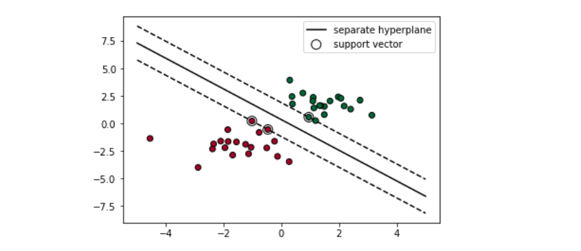
• Support Vector Machine (SVM) is responsible for finding the decision boundary to separate different classes and maximize the margin.
• The goal is to choose a hyperplane with the greatest possible margin (distance) between the hyperplane and any point.
• Only support vectors are important whereas other training examples are ignorable.
  • Support vectors are the data points nearest to the hyperplane. Credit
• By combining the soft margin (tolerance of misclassifications) and kernel trick together, SVM is able to structure the decision boundary for linear non-separable cases:
  • Soft margin tolerates one or few misclassified points.
  • Kernels are functions which transform a low-dimensional space to a higher-dimensional space to make the cases separable.
  • Think of them as a transformer/processor to generate new features by applying the combination of all the existing features.
  • Different kernels functions for different decision boundaries.
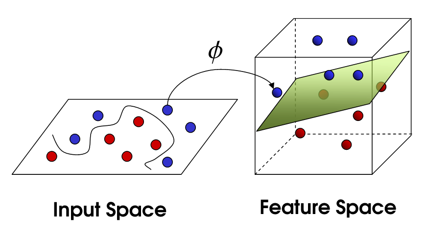
  • The kernel trick avoids explicit transformation of raw representation into feature vector representation (without ever computing the coordinates of the data in that space), which is often computationally cheaper. Credit
• SVM is effective in high-dimensional spaces.
• Works well on smaller cleaner datasets.
• Memory efficient since it uses a subset of training points in the decision function.
• Limitations:
  • Poor performance if the number of features greater than that of samples.
  • Isn’t suited to larger datasets as the training time with SVMs can be high.
  • Less effective on noisier datasets with overlapping classes.
  • SVMs do not provide probability estimates.

Tuning

• SVMs do not require almost any tuning.
• The higher the \(C\), the more penalty, and therefore the less wiggling the decision boundary will be.
• The higher the \(\gamma\), the more influence on the decision boundary, thereby the more wiggling the boundary will be.
• SVC starts to work slower as \(C\) increases. Start with a lower \(C=10\) and multiply it each time by a factor of 10.
• Both libLinear and libSVM have multicore support and can be compiled for fastest speed.
• sklearn wraps them both under the hood but is slower.

Vowpal Wabbit

• Stochastic gradient descent (SGD) gives us practical guidance for training both classifiers and regressors with large amounts of data up to hundreds of GBs (depending on computational resources).
• SGD is a type of online learning algorithm.
  • Online learning is a method of machine learning that stores and processes only one training example at a time sequentially.
  • No need to load all data into memory.
• Since it’s based on one random data point, it’s very noisy:
  • It usually takes dozens of passes over the training set to make the loss small enough.
• VW is more performant than sklearn's SGD models in many aspects.
  • Compiled C++ code.
  • Exploiting multi-core CPUs: parsing of input and learning are done in separate threads.
• With the hashing trick implemented, VW is a perfect choice for working with text data.
• Vowpal Wabbit tutorial: blazingly fast learning