Edit

Recurrect Neural Networks

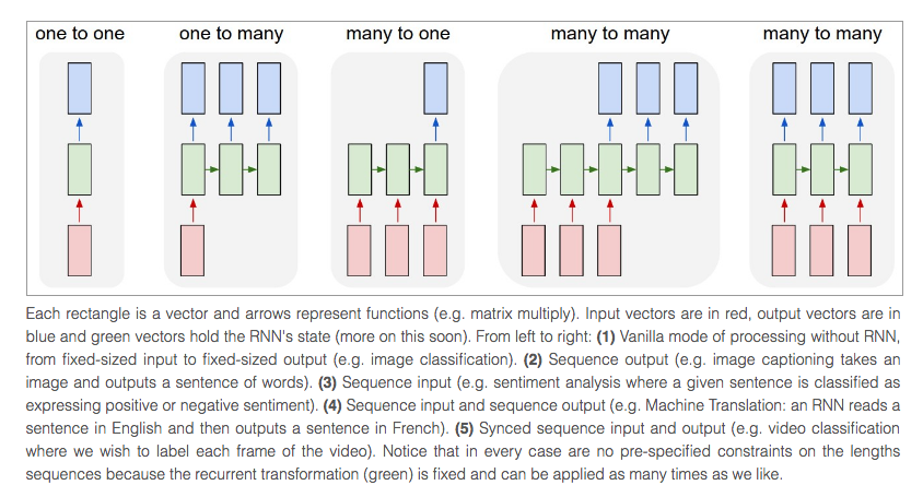
• A glaring limitation of vanilla NNs is that their API is too constrained:
  • They accept fixed-sized vectors as input and as output.
  • These models perform this mapping using a fixed amount of computational steps (e.g. the number of layers in the model).
  • They have no memory of the input they received previously and are therefore bad in predicting what’s coming next.
• If you have to explain RNNs, this is how:

If your neighbor is cooking a dinner each evening and the receipt changes based on the previous one, a vanilla neural network will try to find patterns based on features such as time and mood, while a RNN will try to find sequence patterns and will succeed.

• Unlike feedforward neural networks, RNNs can use their internal state (memory) to process sequences of inputs.

Credit $$\large{h_t=\sigma{(W_h\cdot{[h_{t-1},x_t]}+b_h)}}$$ $$\large{\hat{y_t}=\tanh{(W_yh_t+b_y)}}$$ where \(W_h\): horizontally stacked (learnable) parameters \(W_{t-1}\) and \(W_x\), \([h_{t-1},x_t]\): vertically stacked input vectors \(h_{t-1}\) and \(x_t\)

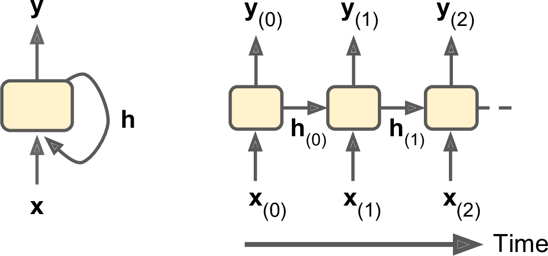
• A recurrent neural network can be thought of as multiple copies of the same network, each passing a message to a successor.
• The outputs in RNNs are just the inputs shifted forward by one, making the RNN a supervised learning model.
• The Unreasonable Effectiveness of Recurrent Neural Networks
• Recurrent Neural Networks (RNN) and Long Short-Term Memory (LSTM)

Turing completeness

• RNNs are Turing-Complete in the sense that they can to simulate arbitrary programs (with proper weights). If training vanilla neural nets is optimization over functions, training recurrent nets is optimization over programs.

Credit

Usage

• Whenever there is a sequence of data and that temporal dynamics that connects the data is more important than the spatial content of each individual frame.
• Even if your data is not in form of sequences, you can still formulate and train powerful models that learn to process it sequentially.
• Evidence suggests the model is good at learning complex syntactic structures (such as XML).

Recurrence

• The most important facet of the RNN is the recurrence.
  • A basic neuron has only connections from his input to his output.
  • The recurrent neuron instead has also a connection from his output again to his input.
• This recurrence indicates a dependence on all the information prior to a particular time.
• RNNs combine the input vector with their state vector with a fixed (but learned) function to produce a new state vector and the output vector. Output vector’s contents are influenced not only by the input you just fed in, but also on the entire history of inputs you’ve fed in in the past.
• Nodes are either:
  • input nodes (receiving data from outside the network)
  • output nodes (yielding results)
  • hidden nodes (that modify the data en route from input to output)

Backpropagation through time (BPTT)

• Since the RNN consists entirely of differentiable operations we can run the backpropagation.
• Within BPTT the error is back-propagated from the last to the first timestep, while unrolling all the timesteps.
  • Note that BPTT can be computationally expensive for a high number of timesteps.

Architectures

Credit

• We can have bidirectional RNNs that feed in the input sequence in both directions by concatenating the outputs of two RNNs, one processing the sequence from left to right, the other one from right to left.

$$\large{\hat{y_t}=\tanh{(W_y\cdot{[\overrightarrow{h_t},\overleftarrow{h_t}]}+b_y)}}$$

where \(\overrightarrow{h_t}\): hidden state of the network pointing right, \(\overleftarrow{h_t}\): hidden state of the network pointing left

• We can also stack these RNNs in layers to make deep RNNs:
  • To process the layers above we first need to iterate over the layers below.
  • In deep RNNs stacking 3 layers is already considered deep and expensive to train.

Pros

• Memorization:
  • The recurrent network can use the feedback connection to store information over time in form of activations.
  • As the time steps increase, the unit gets influenced by larger and larger neighborhood.
  • With that information RNNs can watch short-to-medium-sized regions in the input space.

Credit

• Learn sequential patterns:
  • The RNN can handle sequential data of arbitrary length.
• Furthermore the recurrent connections increase the network depth while they keep the number of parameters low by weight sharing.
• Recurrent connections of neurons are biological inspired and are used for many tasks in the brain.

Cons

• RNN are inefficient and not scalable:
  • If you double the size of the hidden state vector you’d quadruple the amount of FLOPS at each step due to the matrix multiplication.
• RNN and LSTM are memory-bandwidth limited problems:
  • It is easy to add more computational units, but hard to add more memory bandwidth.
• RNNs are not inductive:
  • They memorize sequences extremely well, but they don’t necessarily always show convincing signs of generalizing in the correct way.
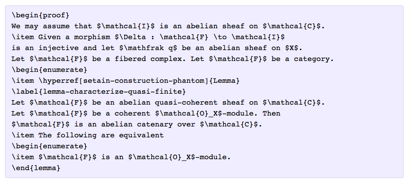
  • For example, the model opens a \begin{proof} environment but then ends it with a \end{lemma}.

Credit

• Problems like exploding and vanishing gradients.
• The recurrent structures are either exploring short-term or long-term temporal structures, but not both simultaneously.
• The fall of RNN / LSTM

Solving gradient problems

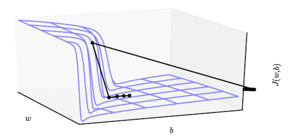
• Vanishing gradients:
  • When gradients are being propagated back in time, they can vanish because they they are continuously multiplied by numbers less than one. This is solved by LSTMs and GRUs, and if you’re using a deep feedforward network, this is solved by residual connections.
• Exploding gradients:
  • This is when they get exponentially large from being multiplied by numbers larger than 1. Gradient clipping will clip the gradients between two numbers to prevent them from getting too large.

Credit

Gating mechanisms

• RNNs suffer from short-term memory:
  • A major problem with gradient descent for standard RNN architectures is that error gradients vanish exponentially quickly with the size of the time lag between important events. RNN model has many local influences, if we not address vanishing gradient problem then RNNs tend not to be very good at capturing long-range dependencies.
• If you are trying to process a paragraph of text to do predictions, RNN’s may leave out important information from the beginning.
• LSTM’s and GRU’s were created as a method to mitigate short-term memory using mechanisms called gates (pipes).

Credit

• These gates can learn which data in a sequence is important to keep or throw away.

Imagine you pick up words like “amazing” and “perfectly balanced breakfast”. You don’t care much for words like “this”, “gave“, “all”, “should”, etc. If a friend asks you the next day what the review said, you probably wouldn’t remember it word for word.

Comparison

• There isn’t a clear winner which one is better:
  • Researchers and engineers usually try both to determine which one works better for their use case.
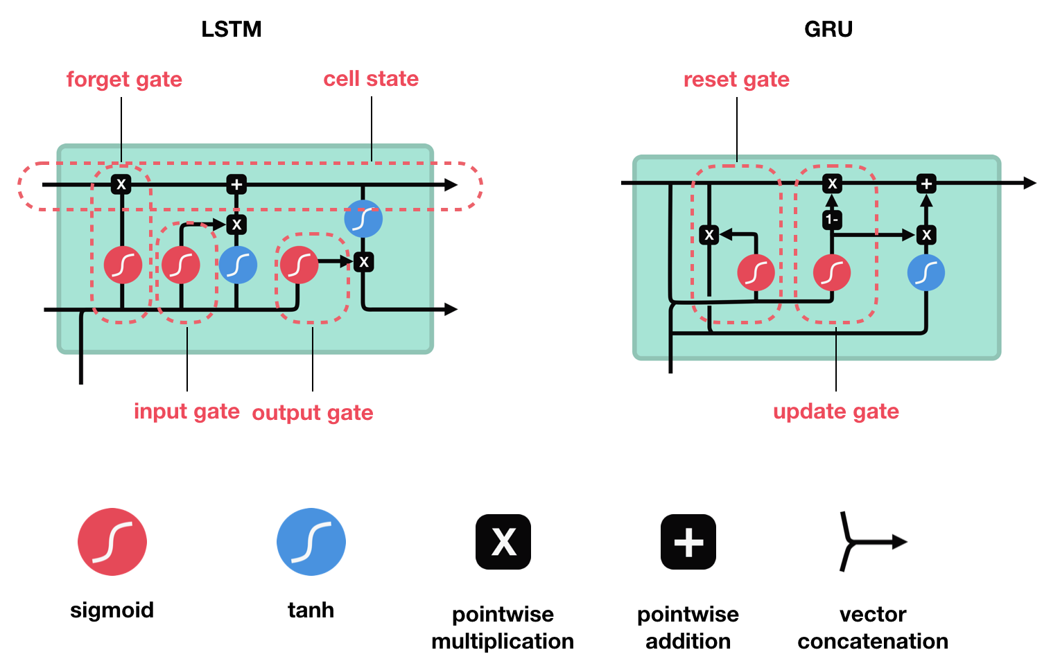
• GRU has fewer tensor operations and parameters than LSTM, as it lacks an output gate.

Credit

Long short-term memory (LSTM)

• Long short-term memory (LSTM) is a deep learning system that avoids the vanishing/exploding gradient problem.
• LSTM’s enable RNN’s to remember their inputs over a long period of time. This is because LSTM’s contain their information in a memory, that is much like the memory of a computer because the LSTM can read, write and delete information from its memory. An interesting analogy can be drawn between memory cells in LSTMs and memory elements in your calculators, storing the numbers you ask it to.
• LSTM can learn tasks that require memories of events that happened thousands or even millions of discrete time steps earlier.
• Understanding LSTM Networks

Gates

• Each LSTM block consists of a forget gate, input gate and an output gate.
• The gates in a LSTM are analog, in the form of sigmoids, meaning that they range from 0 to 1.
• The weights of these connections \(W\) need to be learned during training.
• The input gate \(i_t\) decides what information is relevant to add from the current step. $$\large{i_t=\sigma{(W_i\cdot{[h_{t-1},x_t]}+b_i)}}$$
• The forget gate \(f_t\) decides what is relevant to keep from prior steps. $$\large{f_t=\sigma{(W_f\cdot{[h_{t-1},x_t]}+b_f)}}$$
• The output gate \(o_t\) determines what the next hidden state should be. $$\large{o_t=\sigma{(W_o\cdot{[h_{t-1},x_t]}+b_o)}}$$

Cell state

• The cell state \(c_t\) acts as a transport highway that transfers relative information all the way down the sequence chain.
• You can think of it as the “memory” of the network.
• As the cell state goes on its journey, information get’s added or removed to the cell state via gates. $$\large{\tilde{c_t}=\tanh{(W_c\cdot{[h_{t-1},x_t]}+b_c)}}$$ $$\large{c_t=f_t\odot{c_{t-1}}+i_t\odot{\tilde{c}_{t}}}$$

Hidden state

• The hidden state is the output vector of the LSTM unit. $$\large{h_t=o_t\odot{\tanh(c_{t})}}$$

Gated recurrent unit (GRU)

• Gated recurrent units (GRUs) are a newer gating mechanism in recurrent neural networks.
• GRU’s got rid of the cell state and used the hidden state to transfer information.
• The forget and input gates are combined in a complimentary fashion to reduce the unnecessary complexity in model (reducing recurrent parameters by 33%).
• But LSTM is "strictly stronger" than the GRU as it can easily perform unbounded counting.

Gates

• GRU has two gates, a reset gate and update gate.
• The update gate \(z_t\) decides what information to throw away and what new information to add. $$\large{z_t=\sigma{(W_z\cdot{[h_{t-1},x_t]}+b_z)}}$$
• The reset gate \(r_t\) is another gate is used to decide how much past information to forget. $$\large{r_t=\sigma{(W_r\cdot{[h_{t-1},x_t]}+b_r)}}$$
• But when you combine the 2 operations as a "Coupled Input and Forget Gate" there are similar results compared to the vanilla model.

Hidden state

• The hidden state is the output vector of the GRU unit. $$\large{\tilde{h_t}=\tanh{(W_h\cdot{[r_t\odot{h_{t-1}},x_t]})}}$$ $$\large{h_t=(1-z_t)\odot{h_{t-1}}+z_t\odot\tilde{h_t}}$$